This is a brief summary of ML course provided by Andrew Ng and Stanford in Coursera.
You can find the lecture video and additional materials in
https://www.coursera.org/learn/machine-learning/home/welcome
Coursera | Online Courses From Top Universities. Join for Free
1000+ courses from schools like Stanford and Yale - no application required. Build career skills in data science, computer science, business, and more.
www.coursera.org
Gradient Descents used iteration of minimization of $J(\theta)$ to converge to global minimum.
Solve for optimal value for $\theta$ to the optimal value in one step in Normal Equations.
When you should use normal equation:

Intuition: If 1D $(\theta \in R)$
$J(\theta) = a\theta^2 + b\theta + c $
take derivatives of the above and,
$\frac{\partial}{\partial\theta} J(\theta) = ... = 0$
Solve for $\theta$
$\theta$ is no longer a real number, but n+1 dimensional parameter vector, and,
$J(\theta_0, \theta_1, ..., \theta_m) = \frac{1}{2m} \sum_{i=1}^m (h_{\theta}(x^{(i)}) - y{(i)})^2$
take derivatives of the above and,
$\frac{\partial}{\partial\theta_j} J(\theta) = ... = 0$ (for every j)
Solve for $\theta_0, \theta_1, ..., \theta_n$


Quiz: Suppose you have the training in the table below:
| age (x_1x1) | height in cm (x_2x2) | weight in kg (yy) |
| 4 | 89 | 16 |
| 9 | 124 | 28 |
| 5 | 103 | 20 |
You would like to predict a child's weight as a function of his age and height with the model
weight = $\theta_0 + \theta_1 age + \theta_2 height$
What are X and y?
Answer:
$ X= \left[\begin{array} {rrr} 1 & 4 & 89\\ 1 & 9 & 124 \\ 1 & 5 & 103 \end{array}\right] $ $ y= \left[\begin{array} {rrr} 16 \\ 28 \\ 20 \end{array}\right] $
$\theta = (X^TX)^{-1} X^T y$
$(X^TX)^{-1}$ is the inverse of matrix $X^TX$.
When using normal equation, feature scaling is not really necessary.
Octave: pinv(X'*X)*X'y

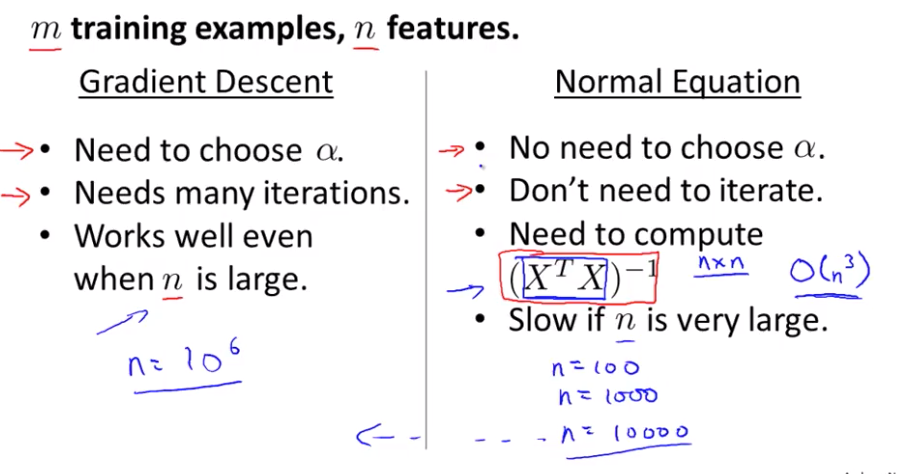
Advantages vs. Disadvantages of Gradient Descent and Normal Equation
Gradient Descent:
- Need to choose $\alpha$ learning rate
- Needs many iterations.
- Works well even when n is large.
Normal Equation:
- No need to choose $\alpha$ learning rate.
- Don't need to iterate.
- Need to compute $(X^TX)^{-1}$ -> $O(n^3)$, slow if n is very large
If N is large, the i might usually use gradient descent because we dont want to pay all in q time. But if n is relatively small, then the normal equation might give you a better way to solve the parameters.
n = 100, 1000 is relatively small and n =10000 is a bit big. (it depends on the machine that you use but n = 10000 can be a standard?)
Lecturer's Note
Gradient descent gives one way of minimizing J. Let’s discuss a second way of doing so, this time performing the minimization explicitly and without resorting to an iterative algorithm. In the "Normal Equation" method, we will minimize J by explicitly taking its derivatives with respect to the θj ’s, and setting them to zero. This allows us to find the optimum theta without iteration. The normal equation formula is given below:
$\theta = (X^TX)^{-1} X^T y$
There is no need to do feature scaling with the normal equation.
The following is a comparison of gradient descent and the normal equation:
| Gradient Descent | Normal Equation |
| Need to choose alpha | No need to choose alpha |
| Needs many iterations | No need to iterate |
| $O (kn^2)$ | $O(n^3)$, need to calculate inverse of $X^T$ |
| Works well when n is large | Slow if n is very large |
With the normal equation, computing the inversion has complexity $O(n^3)$. So if we have a very large number of features, the normal equation will be slow. In practice, when n exceeds 10,000 it might be a good time to go from a normal solution to an iterative process.


