[Machine Learning by Stanford] Classification and Representation - Decision Boundary

This is a brief summary of ML course provided by Andrew Ng and Stanford in Coursera.

You can find the lecture video and additional materials in 

https://www.coursera.org/learn/machine-learning/home/welcome

Coursera | Online Courses From Top Universities. Join for Free

Decision boundary will give a better sense of what the logistic regressions hypothesis function is computing.

Suppose predict "y=1" if $h_{\theta}(x) \geq 0.5$

and predict "y=0" if $h_{\theta}(x) < 0.5$

$g(z) \geq 0.5$, when $z \geq 0$ -> $h_{\theta}(x) \geq 0.5$, when $\theta^T (x) \geq 0$

meaning, if $\theta^T (x) \geq 0$ then y = 1

 

Similarly, 

$g(z) < 0.5$, when $z < 0$ -> $h_{\theta}(x) < 0.5$, when $\theta^T (x) < 0$

meaning, if $\theta^T (x) < 0$ then y = 0

 

To summarize, if we decide to predict whether y=1 or y=0 depending on whether the estimated probability is greater than or equal 0.5, or whether less than 0.5, then that's the same as saying that when we predict y = 1 whenever $\theta^T (x) \geq 0$ 

 

Let's suppose we have a training set like that shown as below. 

Assume that $\theta_0 = -3, \theta_1 = 1, \theta_2 = 1$, or

$\theta = \left[\begin{array} {rrr} -3 \\ 1 \\ 1 \end{array}\right] $,

Let's try to figure out where a hypothesis would end up predicting y equals one and where it would end up y = 0.

We should predict "y=1" if $-3 + x_1 + x_2  \geq 0 $

or $x_1 + x_2 \geq 3 $

 

the equation above in this case, or or $x_1 + x_2 = 3 $ --> $h_{\theta}(x) = 0.5$

makes a decision boundary, and that is the line that separates the region where the hypothesis predicts Y = 1, from the region where the hypothesis predicts that y is equal to zero. 

 

Just to be clear, the decision boundary is a property of the hypothesis including the parameters theta0, theta1, theta2.

Even when dataset is taken away, this decision boundary and the region where we predict y = 1 versus y = 0, that's a property of the hypothesis and of the parameters of the hypothesis and not a property of the data set. 

Later on, we will talk about how to fit the params, and there we will end up using the training set, using our data to determine the value of the parameters. But once we have particular values for the params, that completely defines the decision boundary and we don't actually need to plot a training set in order to plot the decision boundary. 

 

 

Quiz: Consider logistic regression with two features $x_1 , x_2$​. Suppose $ \theta_0 = 5, \theta_1 = -1, \theta_2 = 0 $ , so that $ h_{\theta} (x) = g (5 - x_1) $. Which of these shows the decision boundary of $ h_{\theta} (x) $ ?

 

Answer: Predict Y = 0 if x_1​ is greater than 5.

 

Another example, of crosses to denote my positive examples, and Os to denote my negative examples. 

Assume that $\theta_0 = -1, \theta_1 = 0, \theta_2 = 0, \theta_3 = 1, \theta_4 = 1$ or

$\theta = \left[\begin{array} {rrr} -1 \\ 0 \\ 0 \\ 1 \\ 1 \end{array}\right] $,

 

Indicates, predict "y=1" if $ -1 + x_1^2 + x_2^2 \geq 0$

$x_1^2 + x_2^2 \geq 1$

makes a decision boundary around the circle with radius 1 centered around the origin. 

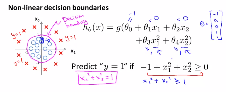
The training set may be used to fit the parameters theta but once you have the params theta, that is what defines the decisions boundary. 

 

 

Lecturer's Note

Decision Boundary

In order to get our discrete 0 or 1 classification, we can translate the output of the hypothesis function as follows:

hθ(x)≥0.5→y=1

hθ(x)<0.5→y=0

The way our logistic function g behaves is that when its input is greater than or equal to zero, its output is greater than or equal to 0.5:

g(z)≥0.5 when z≥0

Remember.

z=0, $e^0$  =1⇒g(z)=1/2

z→∞, e^−∞ →0⇒g(z)=1

z→−∞, e^∞ →∞⇒g(z)=0

 

So if our input to g is $ \theta^T X $, then that means:

hθ(x)=g(θTx)≥0.5, when θTx≥0

 

From these statements we can now say:

θTx≥0⇒y=1

θTx<0⇒y=0

 

The decision boundary is the line that separates the area where y = 0 and where y = 1. It is created by our hypothesis function.

Example:

In this case, our decision boundary is a straight vertical line placed on the graph where $ x_1 = 5 $, and everything to the left of that denotes y = 1, while everything to the right denotes y = 0.

Again, the input to the sigmoid function g(z) (e.g. $ \theta^T X $ ) doesn't need to be linear, and could be a function that describes a circle (e.g.  $ z=  \theta_0 + \theta_1 x_1^2 + \theta_2 x_2^2 $ ) or any shape to fit our data.