[Machine Learning by Stanford] Solving the Problem of Overfitting - Cost Function

This is a brief summary of ML course provided by Andrew Ng and Stanford in Coursera.

You can find the lecture video and additional materials in 

https://www.coursera.org/learn/machine-learning/home/welcome

Coursera | Online Courses From Top Universities. Join for Free

Suppose we penalize and make $\theta_3, \theta_4$ really small. 

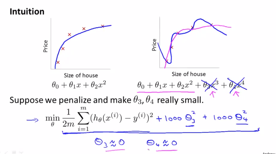
then there exist only a tiny contributions from $\theta_3, \theta_4$

 

Regularization

Small values for parameters  $\theta_0, \theta_1, ...,  \theta_n$

- "Simpler" hypothesis

- Less prone to overfitting

Housing: we don't which feature is $\theta_3, or \theta_4$

- Features: $x_0, x_1, ...,  x_100$

- params: $\theta_0, \theta_1, ...,  \theta_100$

 

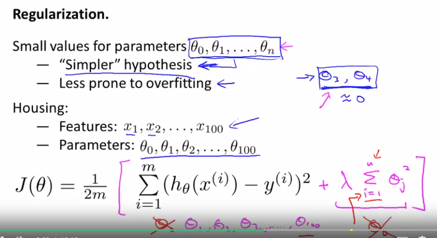
In regularization, we are going to take the cost function, modify it to shrink all of the params by adding the regularization term at the end. 

By convention this regularization term does not include i = 0. but in practice, that won't really matter. 

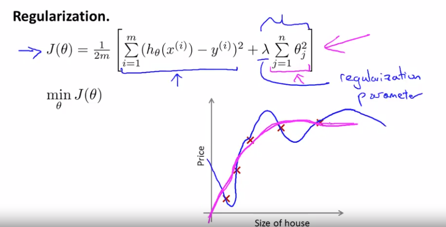
$\lambda$ is a regularization parameter, which controls a trade off between two different goals.

1. we would like to fit a training set well. (what usual cost fucntion does)

2. we want to keep the parameter small.  (terms after lambda) 

 

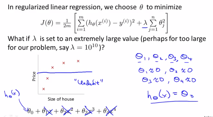
Quiz:

a. Algorithm works fine; setting \lambdaλ to be very large can't hurt it.

b. Algorithm fails to eliminate overfitting.

c. Algorithm results in underfitting (fails to fit even the training set).

d. Gradient descent will fail to converge.

 

Answer: c

 

If $\lambda$ is set to an extremely large value (perhaps for too large for our problem, say $\lambda = 10^10$?

We will end up with all of these params close to zero. and provide a flat horizontal line to the data. 

Therefore a good choice for regularization parameter lambda is needed. 

 

Lecuter's Note:

Cost Function

 

If we have overfitting from our hypothesis function, we can reduce the weight that some of the terms in our function carry by increasing their cost.

Say we wanted to make the following function more quadratic:

$ \theta_0 + \theta_1 x + \theta_2 x^2 + \theta_3 x^3 + \theta_4 x^4$

 

We'll want to eliminate the influence of $ \theta_3 x^3, \theta_4 x^4$. Without actually getting rid of these features or changing the form of our hypothesis, we can instead modify our cost function:

 

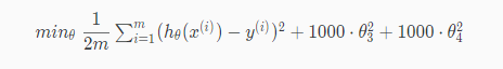
We've added two extra terms at the end to inflate the cost of $ \theta_3 x^3, \theta_4 x^4$. Now, in order for the cost function to get close to zero, we will have to reduce the values of $ \theta_3 x^3, \theta_4 x^4$ to near zero. This will in turn greatly reduce the values of$ \theta_3 x^3, \theta_4 x^4$ in our hypothesis function. As a result, we see that the new hypothesis (depicted by the pink curve) looks like a quadratic function but fits the data better due to the extra small terms $ \theta_3 x^3, \theta_4 x^4$.

 

We could also regularize all of our theta parameters in a single summation as:

The λ, or lambda, is the regularization parameter. It determines how much the costs of our theta parameters are inflated.

 

Using the above cost function with the extra summation, we can smooth the output of our hypothesis function to reduce overfitting. If lambda is chosen to be too large, it may smooth out the function too much and cause underfitting. Hence, what would happen if λ=0 or is too small ?  

(underfitting occurs)