[Machine Learning by Stanford] Solving the Problem of Overfitting - Regularized Linear Regression

This is a brief summary of ML course provided by Andrew Ng and Stanford in Coursera.

You can find the lecture video and additional materials in 

https://www.coursera.org/learn/machine-learning/home/welcome

Coursera | Online Courses From Top Universities. Join for Free

Two learning algorithms, gradient descent and normal equation. 

we will take these two algorithms and generalize themn to the case of regularized linear regression. 

 

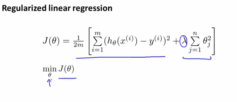
We would like to find theta that minimizes the regularized cost function J, 

 

For regularized linear regression, we penalize the params, $\theta_1, \theta_2 , ... $ except $\theta_0$. 

So should treat $\theta_0$ slightly different from others. 

Implement below, then you will have the gradient descent for trying to minimize the regularized cost function J. 

the terms in bracket is a partial derivative with respect to J of theta using the new definition of J of theta with the regularization term. 

 

 

Quiz: 

Suppose you are doing gradient descent on a training set of m>0 examples, using a fairly small learning rate α>0 and some regularization parameter λ>0. Consider the update rule:

Which of the following statements about the term (1−αλ/m​) must be true?

a. 1−αλ/m​>1

b. 1−αλ/m​=1

c. 1−αλ/m​<1

None of the above.

 

Answer: c

 

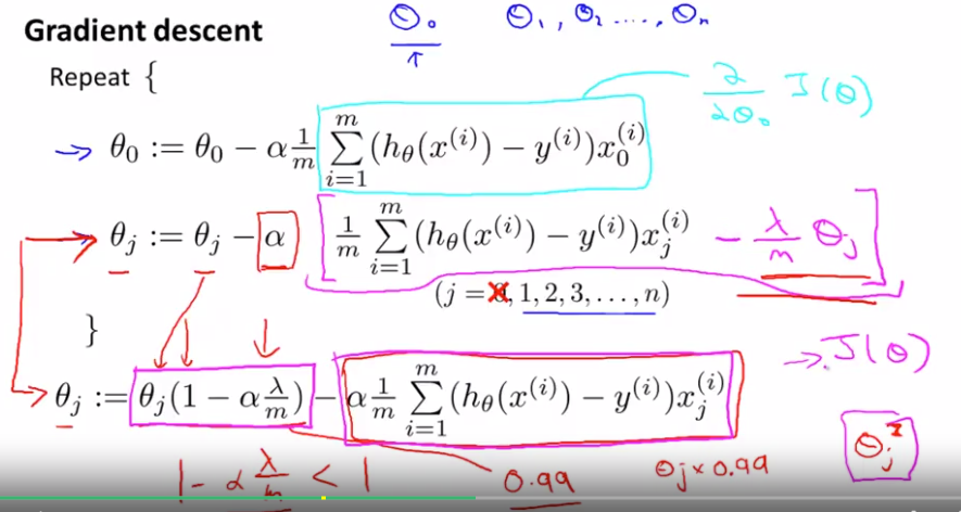
$ (1- \alpha\frac{\lambda}{m}) $ usually should be a little less than 1. (assume 0.99 here) 

Thus, $\theta_j$ * 0.99 makes thteta j a bit smaller at each iteration. 

and the second term is the original gradient descent that we used to have. 

So when regularization, what we are doing is on every iteration we are multiplying theta j by a number that is a little bit less than one, so it is shrinking the parameter a little bit, and performs similiar update as before. 

 

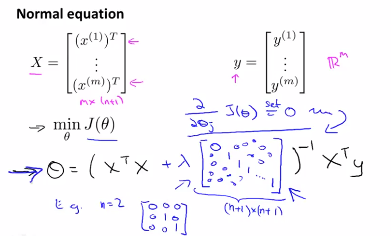
For normal equation, where what we did was we created the design matrix X where each row corresponded to a separate training example. and we created vector y, so this is a vector, which contains the labels from my training set. (X is m by (n+1) dimensional matrix, and y is an m dimensional vector) 

In order to minimize the cost function J, we found that, one way to do so, is to set

$\theta = (X^X )^{-I} X^T y $

What value for theta does is that it minimizes the cost function J of theta when we were not using regularization. Now that we are using regularization, 

$\theta = (X^X + \lambda []  )^{-I} X^T y $

 

Using this, you will be able to avoid overfitting even if you have lots of features in a relatively small training set. 

 

The issue of non-invertibility (optinal/ advanced)

If you have fewer examples than features than the matrix is non-invertible (singular/ degenerate). 

pinv in matlab will also take care of this issue, as it did earlier with non-invertible case. (search for the topic in this blog)

 

 

Lecturer's Note

Regularized Linear Regression

We can apply regularization to both linear regression and logistic regression. We will approach linear regression first.

Gradient Descent

We will modify our gradient descent function to separate out \theta_0θ0​ from the rest of the parameters because we do not want to penalize θ0​.

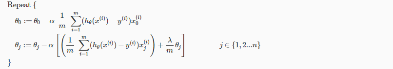
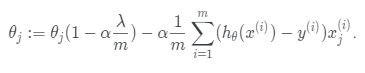
The term $\frac{\lambda}{m} \theta_j $​ performs our regularization. With some manipulation our update rule can also be represented as:

$\theta_j := \theta_j(1-\alpha \frac{\lambda}{m}) - \alpha \frac{1}{m} \sum_{i=1}^m (h_\theta (x^{(i)} - y^{(i)} x_j^{(i)}$

The first term in the above equation, $\theta_j(1-\alpha \frac{\lambda}{m}) $ will always be less than 1. Intuitively you can see it as reducing the value of θj​ by some amount on every update. Notice that the second term is now exactly the same as it was before.

Normal Equation

Now let's approach regularization using the alternate method of the non-iterative normal equation.

To add in regularization, the equation is the same as our original, except that we add another term inside the parentheses:

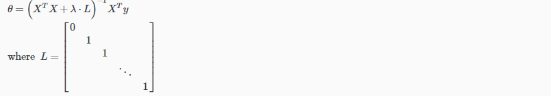
L is a matrix with 0 at the top left and 1's down the diagonal, with 0's everywhere else. It should have dimension (n+1)×(n+1). Intuitively, this is the identity matrix (though we are not including x0​), multiplied with a single real number λ.

Recall that if m < n, then $X^T X$ is non-invertible. However, when we add the term λ⋅L, then$X^T X + \lambda * L $becomes invertible.