This is a brief summary of ML course provided by Andrew Ng and Stanford in Coursera.
You can find the lecture video and additional materials in
https://www.coursera.org/learn/machine-learning/home/welcome
Coursera | Online Courses From Top Universities. Join for Free
1000+ courses from schools like Stanford and Yale - no application required. Build career skills in data science, computer science, business, and more.
www.coursera.org
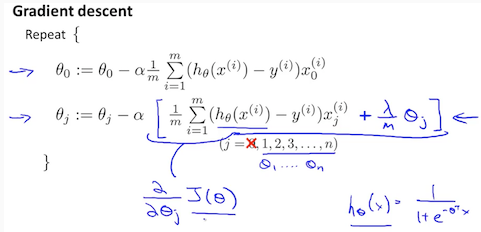
Adapt both gradient descent and the more advanced optimization techniques in order to have them work for regularized logistic regression.
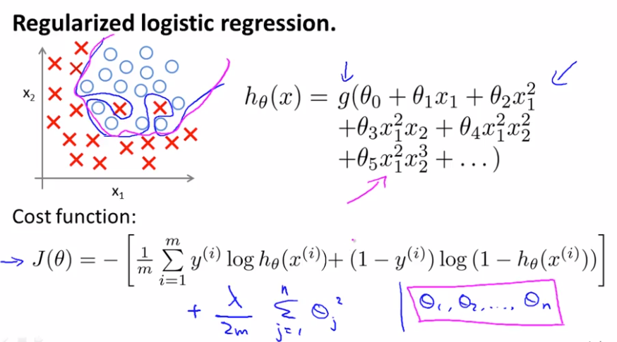
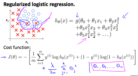
With a lot of features, you can end up with overtfitting for logistic regression problems.
New cost function below will give you the effect that even though you are fitting a very high order polynomial with a lot of params, so long as you apply regularization, and keep the params small, you are more likely to get a decision boundary, more reasonably separating the positive and the negative examples.
Quiz: When using regularized logistic regression, which of these is the best way to monitor whether gradient descent is working correctly?

Answer: c
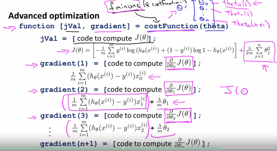
Cost functions need to return were first J-val (need to compute the cost function J of theta)
Lecturer's Note
Regularized Logistic Regression
We can regularize logistic regression in a similar way that we regularize linear regression. As a result, we can avoid overfitting. The following image shows how the regularized function, displayed by the pink line, is less likely to overfit than the non-regularized function represented by the blue line:
Cost Function
Recall that our cost function for logistic regression was:
$J(\theta) = - \frac{1}{m}\sum_{i=1}^m [y^{(i)} log (h_{\theta} (x^{(i)}) + (1-y^{(i)}) log ( 1 - h_{\theta}(x^{(i)}))]$
We can regularize this equation by adding a term to the end:

The second sum, $\sum_{j=1}^n \theta_j^2$ means to explicitly exclude the bias term, θ0. I.e. the θ vector is indexed from 0 to n (holding n+1 values, θ0 through θn), and this sum explicitly skips θ0, by running from 1 to n, skipping 0. Thus, when computing the equation, we should continuously update the two following equations: