[Machine Learning by Stanford] Cost Function and Back-propagation - Backpropagation Algorithm

This is a brief summary of ML course provided by Andrew Ng and Stanford in Coursera.

You can find the lecture video and additional materials in 

https://www.coursera.org/learn/machine-learning/home/welcome

Coursera | Online Courses From Top Universities. Join for Free

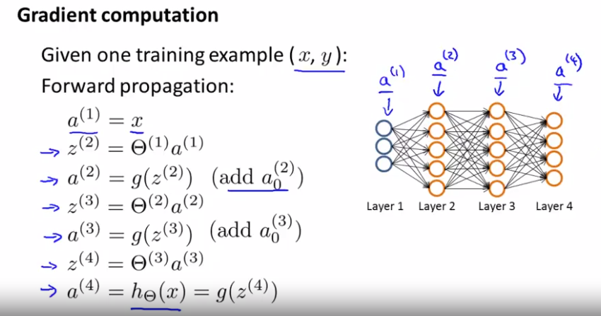
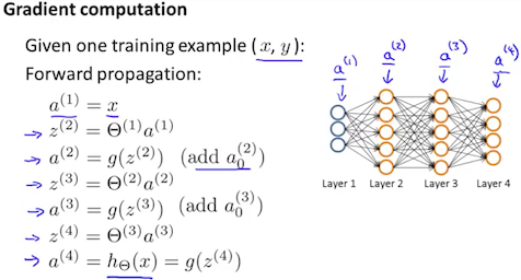
First, we apply forward propagation in order to compute whether a hypotheses actually outputs given the input.

Concretely, a(1) is the activation values of the first layer that was the input layer. (set that to x)

z(2) equals $theta^{(1)} a^{(1)}$ , 

a(2) is the sigmoid activation function applied to z(2) and this would give the activations for the first middle layer (layer 2 for the network) and we also add those bias terms. 

Next, we apply 2 more steps of this forward propagation to compute a(3), and a(4) (outputo f the hypothesis) 

This is our vectorized implementation of forward propagation and it allows us to compute the activation values for all of the neurons.  

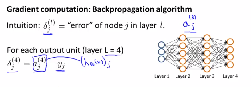
Next, in order to compute the derivatives, we are going to use an algorithm called back-propagation. 

Intuition: $\delta_j^{(l0} = $ "error" of node j in layer l. 

$a_j^{(l)}$ activation of the jth unit in layer l. 

delta term is in some sense going to capture our error in the activation.

 

For example, the neural network below shows 4 layers.

$\delta_j{(4)} = a_j^{(4)} - y_i $

activation of that unit - actual value in the training example. 

 

In vectorized implementation, whose dimension is equal to the number of output units in our network. 

$\delta^{(4)} = a^{(4)} - y$

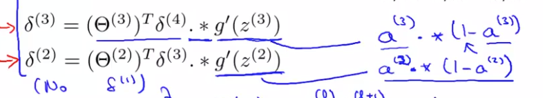
and we compute $\delta^{(3)}, \delta^{(2)}$

.* is an element-wise multiplication. 

derivative of g function of the activation function, which i am denoting by g'. 

 

Finally, there is no $\delta^{(1)}$ term, because the first layer corresponds to the input layer and that is just the features we observed in our dataset. So that does not have any error associated with that and we don't want to try to change those values. 

 

The name back-propagation comes from the fact taht we start by computing the delta term for the output layer and then we go back a layer and compute the delta terms for third hidden layer and then we go back nother step to compute delta. So we are sort of back-propagating the errors from the output layer to layer 3 to layer 2, henced name back propagation. 

 

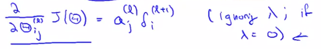
The derivation is surprisingly compliacted, surprisingly involved but if you just do this few steps of computation, it is possible to prove viral frankly some what complicated mathematical proof. It is possible to prove that if you ignore regularization then the partial derivative you want are exactly given by the activations and these delta terms. 

 

 

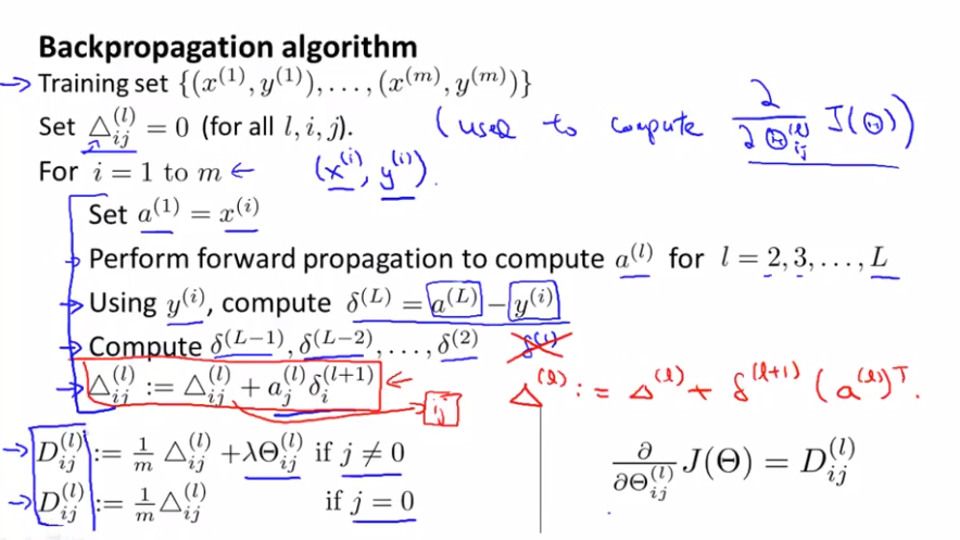
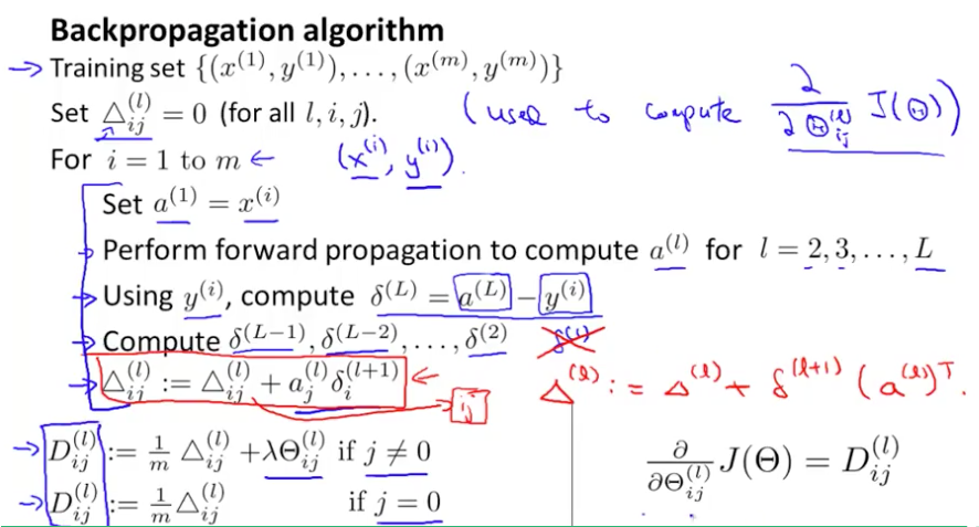
Suppose we have m training examples,

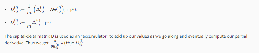
1. set $\Delta_{ij}^{(l)}$ = 0 (for all l, i, j) --> will be used to compute $\frac{\partial}{\partial\theta^{(l)}} J(\theta)$

- delta will be used as an accumulator that will slowly add things in order to compute these partial derivatives. 

2. Loop through the training sets,

for i = 1 to m  <-- $(x^{(i)}, y^{(i)})$

  set $a^{(1)} = x^{(1)}$

  perform forward propagation to compute $a^{(l)} for l = 2, 3, ... , L$

  Using $y^{(i)}$, compute $\delta^{(L)} = a^{(L)} - y^{(i)}$ // compute the error term $a^{(L)}$ is a hypotheses output

  Compute $\delta^{(L-1)}, \delta^{(L-2)}, ..., \delta^{(2)}$ // use back-propagation algorithm

  $\Delta_{ij}^{(l)} := \Delta_{ij}^{(l)} + a_j^{(l)}\delta^{(l+1)}$

* note that there is no delta one, because we don't associate an error term with the input layer. 

 

You can do vectorized implementation for the accumulated delta as below:

 

3. D term is exactly the partial derivative of the cost function with respect to each of your parameters and so you can use those in either gradient descent or the one of the advanced optimization algorithms. 

case of j=0 corresponds to the bias terms, then we don't need the extra regularization term. 

 

 

Quiz: Suppose you have two training examples $(x^{(1)}, y^{(1)})$ and $(x^{(2)}, y^{(2)})$ . Which of the following is a correct sequence of operations for computing the gradient? (Below, FP = forward propagation, BP = back propagation).

a. FP using $x^{(1)}$ followed by FP using $x^{(2)}$ . Then BP using $y^{(1)}$ followed by BP using $y^{(2)}$.

b. FP using $x^{(1)}$  followed by BP using $y^{(2)}$. Then FP using $x^{(2)}$  followed by BP using $y^{(1)}$.

c. BP using $y^{(1)}$ followed by FP using $x^{(1)}$ . Then BP using $y^{(2)}$ followed by FP using $x^{(2)}$ .

d. FP using $x^{(1)}$  followed by BP using $y^{(1)}$. Then FP using $x^{(2)}$  followed by BP using $y^{(2)}$.

 

answer: d

 

Lecturer's Note

Backpropagation Algorithm

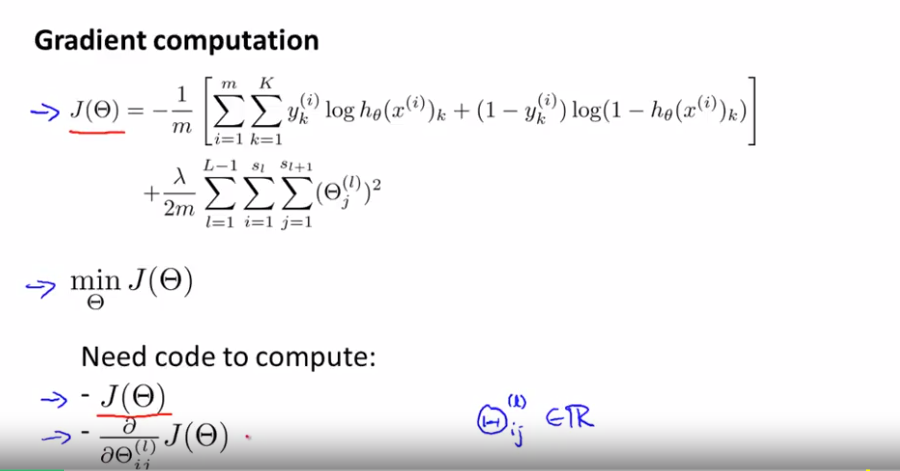
"Backpropagation" is neural-network terminology for minimizing our cost function, just like what we were doing with gradient descent in logistic and linear regression. Our goal is to compute:

minΘJ(Θ)

That is, we want to minimize our cost function J using an optimal set of parameters in theta. In this section we'll look at the equations we use to compute the partial derivative of J(Θ):

$\frac{\partial}{\partial\theta_{i,j}^{(l)}} J(\theta)$

 

To do so, we use the following algorithm:

Back propagation Algorithm

Given training set $(x^{(1)}, y^{(1)}) ... (x^{m}, y^{m})$

- set $\Delta_{i,j}^{(l)}$ := 0 for all (l,i,j), (hence you end up having a matrix full of zeros)

For training example t =1 to m:

1. Set $a^{(1)} := x^{(t)}a(1) := x(t)$
2. Perform forward propagation to compute $a^{(l)} for l = 2, 3, ..., L$

3. Using $y^{(t)}$, compute $\delta^{(L)} = a^{(L)} - y^{(t)}$

Where L is our total number of layers and $a^{(L)}$ is the vector of outputs of the activation units for the last layer. So our "error values" for the last layer are simply the differences of our actual results in the last layer and the correct outputs in y. To get the delta values of the layers before the last layer, we can use an equation that steps us back from right to left:

 

4. Compute $\delta^{(L-1)}, \delta^{(L-2)}, ..., \delta^{(2)}$ using $\delta^{(l)} = ((\theta^{(l)})^T \delta^{(l+1)}) .* a^{(l)} .* (1 - a^{(l)})$

The delta values of layer l are calculated by multiplying the delta values in the next layer with the theta matrix of layer l. We then element-wise multiply that with a function called g', or g-prime, which is the derivative of the activation function g evaluated with the input values given by $z^{(l)}$.

The g-prime derivative terms can also be written out as:

$g'(z^{(l)}) = a^{(l)} .* (1 - a^{(l)})$

 

5. $\Delta_{i,j}^{(l)} := \Delta_{i,j}^{(l)} + a_j^{(l)} \delta_i^{(l+1)}$ or with vectorization, $\Delta^{(l)} := \Delta^{(l)} + \delta^{(l+1)} (a^{(l)})^T$

Hence we update our new $\Delta$ matrix.