[Machine Learning by Stanford] Backpropagation in Practice - Gradient Checking

This is a brief summary of ML course provided by Andrew Ng and Stanford in Coursera.

You can find the lecture video and additional materials in 

https://www.coursera.org/learn/machine-learning/home/welcome

Coursera | Online Courses From Top Universities. Join for Free

There could be a case where you might just wind up with a neural network that has a higher level of error than you would with a bug free implementation. and you might just not know that there was this subtle bug that was giving you worse performance. 

 

Through gradient checking, you can eliminate almost all of these problems. and if you do this, it will help you make sure and sort of gain high confidence that your implementation of forward prop and back prop or whatever is 100% correct. 

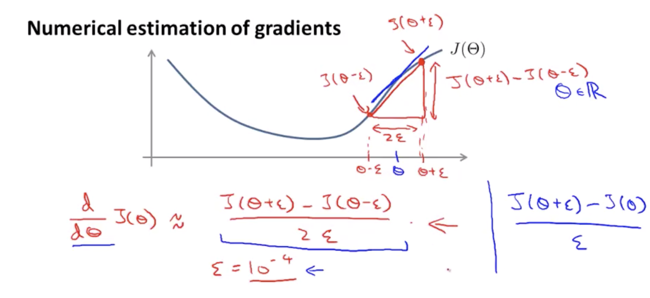
Left formula is called a two-sided difference, and the right one is called one-sided difference. 

With an octave, call to compute gradApprox, which is going to be our approximation derivative as just the equation of twosided difference. This will give you a numerical estimate of the gradient at that point. 

 

Quiz: Let $j(\theta) = \theta^3$. Furthermore, let $\theta =  1, \epsilon = 0.01.$ you use the formula

$\frac{j(\theta+\epsilon) - j(\theta-\epsilon)}{2\epsilon}$ to approximate the derivative. What value do you get using this approximation? (When $\theta=1$, the true, exact derivative $\frac{\partial}{\partial\theta} J(\theta) =3$). 

 

Answer: 3.0001

 

We considered the case of when theta was a real number. 

Let's look at a case of when theta is a vector parameter. 

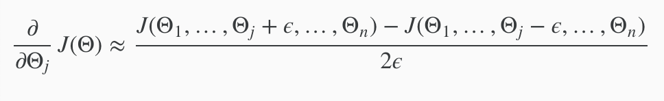
The partial derivative of a cost function with respect to the first parameter, theta one, that can be obtained by taking J and increasing theta one. The partial derivative respect to the second param theta two, is again this except that you would take j of increasing theta two by epsilon, decreasiing theta two by epsilon and so on down to the derivative with respect of theta n would give you increase and decrease theta n by epsilon.

 

So these equations give you a way to numerically approximate the partial derivative of J/ with respect to any one of your param theta i. 

With octave, 

  for i = 1; n,   //n is a dimension of the parameter vector theta (unrolled version) 

    thetaPlus = theta; 

    thetaPlus(i) = thetaPlus(i) + EPSILON;

    thetaMinus = theta

    thetaMinus(i) = thetaMinus(i) - EPSILON;

    gradApprox(i) = (J(thetaPlus) - J(thetaMinus)) / (2*EPSILON); 

  end;

Check gradApprox if its equal to DVec (from back propagation, which is a relatively efficient way to compute a derivative or a partial derivative of a cost function with respect to all our params)

If those values are approximately similiar, then I can be more confident that i am computing those derivatively correctly. 

Implementation Note: 

- implement backprop to compute DVec (unrolled D(1), D(2), D(3)).

- implement numerical gradient descent check to compute gradApprox

- Make sure they give similar values

- Turn off gradient checking. Using backprop code for learning. 

 

Important

- be sure to disable your gradient checking code before training your classifier. I/f you run numerical gradient computation on every iteration of gradient descent (or in the inner loop of costFunction, your code will be very slow. 

 

* Backprop is much more computationally efficient way of computing for derivatives. So once you have verified the implementation of back props, you should turn off gradient checking and just stop using that. 

Quiz: What is the main reason that we use the backpropagation algorithm rather than the numerical gradient computation method during learning?

a. The numerical gradient computation method is much harder to implement.

b. The numerical gradient algorithm is very slow.

c. Backpropagation does not require setting the parameter EPSILON.

d. None of the above.

 

Answer: b

 

Lecturer's Note:

Gradient Checking

Gradient checking will assure that our backpropagation works as intended. We can approximate the derivative of our cost function with:

 

$\frac{\partial}{\partial\theta} J(\theta) \approx \frac{J(\theta+\epsilon) - J(\theta-\epsilon)}{2\epsilon}$

With multiple theta matrices, we can approximate the derivative with respect to $\theta_j$ as follows:

A small value for ϵ (epsilon) such as ϵ=10−4, guarantees that the math works out properly. If the value for ϵ is too small, we can end up with numerical problems.

Hence, we are only adding or subtracting epsilon to the Θj matrix. In octave we can do it as follows:

We previously saw how to calculate the deltaVector. So once we compute our gradApprox vector, we can check that gradApprox ≈ deltaVector.

Once you have verified once that your backpropagation algorithm is correct, you don't need to compute gradApprox again. The code to compute gradApprox can be very slow.