[Machine Learning by Stanford] Backpropagation in Practice -Random Initialization

This is a brief summary of ML course provided by Andrew Ng and Stanford in Coursera.

You can find the lecture video and additional materials in 

https://www.coursera.org/learn/machine-learning/home/welcome

Coursera | Online Courses From Top Universities. Join for Free

The idea of random initialization

 

When you are running an algorithm of gradient descent, or also the advanced optimization algorithms, we need to pick some inital value for the params theta. So for the optimization algorithm, it assumes you will pass it some initial value for the param theta. 

Consider a gradient descent. For that, we will also need to initialize theta to something, and then we can slowly take steps to go downhill using gradient descent. To go downhill, to minimize the function j of theta. 

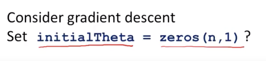
- Can we set the initial value of theta to the vector of all zeros? Wheras this worked okay when we were using logistic regression, initializing all of your params to zero actually does not work when you are trading on your own network. 

What it means to have zeros for initializing all of the params to be zero, is to have the colored edges to hidden units are going to be computed the same function of the inputs. And thus you would end up with for every one of your training examples, 

$a_1^{(2)} = a_2^{(2)}, also \delta_1^{(2)} = \delta_2^2{(2)}$.

$\theta_{01}^{(1)} = \theta_{(02}^

--> After each update,parameters corrsponding to input going into each of two hidden units become identical

 

Imagine if you have many, many hidden units, then all of your hidden units are computing the exact same feature or

all of your hidden units are computing the exact same function of the input and this is a highly redundant representation because you find the logistic progression unit, it really has to see only one feature because all of these are the same. 

 

In order to get around this problem, the way we initialize the parameters of a neural network therefore is with random initialization. 

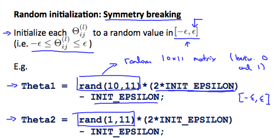
The method we use the above is called the problem of symmetric ways, that is the ways are being the same. So this random initialization is how we perform symmetric breaking. 

 

1. Initialize each value of theta to a random number between $-\epsilon, \epsilon$

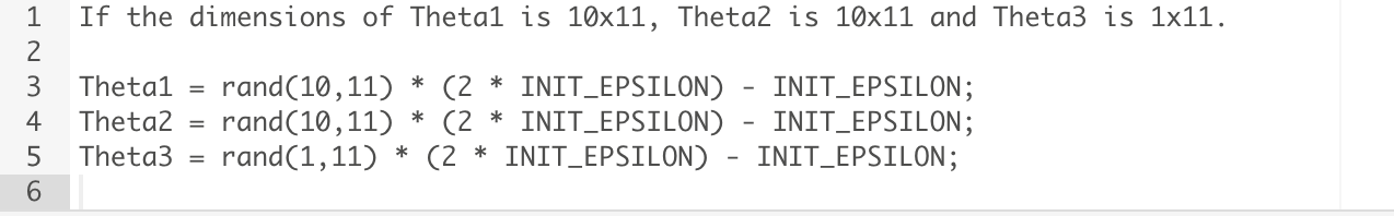
e.g., theta1 = rand(10,11) * (2*INIT_EPSILON) - INIT_EPSILON; 

theta2 = rand(10,11) * (2*INIT_EPSILON) - INIT_EPSILON; 

* note this epsilon value is different from the one from gradient checking. 

 

Quiz: Consider this procedure for initializing the parameters of a neural network:

1. Pick a random number r = rand(1,1) * (2 * INIT_EPSILON) - INIT_EPSILON;
2. Set Θ(l)ij=r for all i,j,li,j,l.

Does this work?

a. Yes, because the parameters are chosen randomly.

b. Yes, unless we are unlucky and get r=0 (up to numerical precision).

c. Maybe, depending on the training set inputs x(i).

d. No, because this fails to break symmetry.

 

Answer: d

 

So to summarize, to create a neural network what you should do is randomly initialize the waves to small values close to zero between -epsilon and + epsilon. 

And then implement back propagation

Do gradient checking. 

Use either gradient in descent or advanced optimization algorithms to try to minimize j (theta) as a function of the parameters theta starting from just randomly chosen initial value for the params.

And by doing symmetric breaking, which is this process, hopefully gradient descent or the advanced optimization algo will be able to find a good value of theta. 

 

Lecturer's Note:

Random Initialization

Initializing all theta weights to zero does not work with neural networks. When we backpropagate, all nodes will update to the same value repeatedly. Instead we can randomly initialize our weights for our Θ matrices using the following method:

Hence, we initialize each Θ(l)ij to a random value between[−ϵ,ϵ]. Using the above formula guarantees that we get the desired bound. The same procedure applies to all the Θ's. Below is some working code you could use to experiment.

 

rand(x,y) is just a function in octave that will initialize a matrix of random real numbers between 0 and 1.

(Note: the epsilon used above is unrelated to the epsilon from Gradient Checking)