[Machine Learning by Stanford] Backpropagation in Practice - Putting it Together

This is a brief summary of ML course provided by Andrew Ng and Stanford in Coursera.

You can find the lecture video and additional materials in 

https://www.coursera.org/learn/machine-learning/home/welcome

Coursera | Online Courses From Top Universities. Join for Free

When training a neural network, the first thing you need to do is pick some network architecture.

and by architecture, I just mean connectivity pattern between the neurons. So we might choose between say, a nerual netwrok with three inputs units and five hidden units and four output units versus one of 3,5 hidden, 5hidden, 4 output and here are 3,5,5,5 units in each of three hidden layers and for open units, and so these choices of how many hidden units in each layer and how many hidden layers, those are architecture choices. 

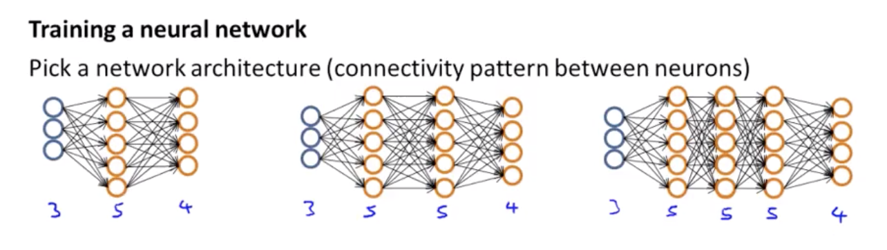
How do you make these choices?

No. of input units: Dimension of features $x^{(i)}$

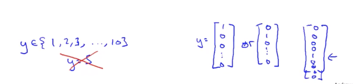
No. output units: Number of classes

Reasonable Derfault: 1 hidden layer, or if >1 hidden layer, have same no of hidden units in every layer (usually the more number of hidden units the better) 

 

 

Training a neural network

1. Randomly initialize weights (small values near to zero)

2. Implement forward propagation to get $h_{\theta}(x^{(i)})$ for any $x^{(i)}$

3. Implement code to compute cost function $J(\theta)$

4. Implement backprop to compute partial derivatives $\frac{\partial}{\partial\theta_{jk}^{(i)}} J(\theta)$

 

To implement back prop,

for i = 1:m  (loop over training examples)

  perform forward propagation and backpropagation using example $(x^{(i)}, y^{(i)})$

  (get activations $a^{(l)}$ and delta terms $\delta^{(l)}$ for l= 2, ..., L).

5. Use gradient checking to compare $\frac{\partial}{\partial\theta){jk}^{(l)}} J(\theta) $ computed using backpropagation vs. using numerical estimate of gradient of $J(\theta)$. Then disable gradient checking code. (gradient checking is computationally expensive)

6. Use gradient descent or advanced optimization method with propagation to try to minimize $J(\theta)$ as a function of params $\theta$. 

for neural network $\j(\theta)$ is non-convex, theoretically be susceptible to local minima, and in fact algorithms like gradient descent and the advanced optimization methods can get stuck in local optima. But in practice this is not usually a huge problem and even though we cannot guarantee that these algorithms will find a global optimum, usually algorithms like gradient descent will do a very good job minimizing this cost function j of theta and get a very good local minimum, even if it does not get to the global optimum. 

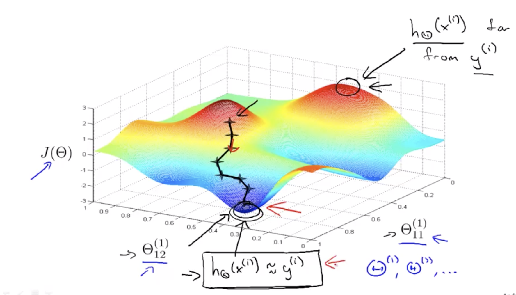
Finally, gradient descents for a neural network might still seem a little bit magical. 

The cost function $J(\theta)$measures how well the neural network fits the training data. So if you take a point, where $J(\theta)$ is pretty low, this corresponds to a setting of the params, where for most of the training examples, the output of the hypotheses, that may be pretty close to $y^{(i)}$ and if this is true, then that's what causes my cost function to be prety low. 

Whereas in contrast, if you were to take a value in some high position, the output of the neural network is far from the actual value $y^{(i)}$. So it is not fitting the training set well, whereas points with low values of the cost function corresponds to where j of theta is low, and therefore corresponds to where the neural network happens to be fitting the training set well, because this is what is needed to be true in order for j of theta to be small. 

So what gradient descent does is we will start from some random initial point  and it will repeatedly go downhill. 

And so what back propagation is doing is computing the direction of the gradient, and what gradient descent is doing is it is taking little steps downhill until hopefully it gets to a good local optimum. it is trying to find a value of the parameters where the output values in the neural network closely matches the values  of the $y^{(i)}$'s observed in the training set. 

Quiz: Suppose you are using gradient descent together with backpropagation to try to minimize J(Θ) as a function of Θ. Which of the following would be a useful step for verifying that the learning algorithm is running correctly?

a. Plot J(Θ) as a function of Θ, to make sure gradient descent is going downhill.

b. Plot J(Θ) as a function of the number of iterations and make sure it is increasing (or at least non-decreasing) with every iteration.

c. Plot J(Θ) as a function of the number of iterations and make sure it is decreasing (or at least non-increasing) with every iteration.

d. Plot J(Θ) as a function of the number of iterations to make sure the parameter values are improving in classification accuracy.

 

Answer: c

 

Lecturer's Note

Putting it Together

First, pick a network architecture; choose the layout of your neural network, including how many hidden units in each layer and how many layers in total you want to have.

• Number of input units = dimension of features $x^{(i)}$
• Number of output units = number of classes
• Number of hidden units per layer = usually more the better (must balance with cost of computation as it increases with more hidden units)
• Defaults: 1 hidden layer. If you have more than 1 hidden layer, then it is recommended that you have the same number of units in every hidden layer.

Training a Neural Network

1. Randomly initialize the weights
2. Implement forward propagation to get hΘ(x(i)) for any $x^{(i)}$
3. Implement the cost function
4. Implement backpropagation to compute partial derivatives
5. Use gradient checking to confirm that your backpropagation works. Then disable gradient checking.
6. Use gradient descent or a built-in optimization function to minimize the cost function with the weights in theta.

When we perform forward and back propagation, we loop on every training example:

The following image gives us an intuition of what is happening as we are implementing our neural network:

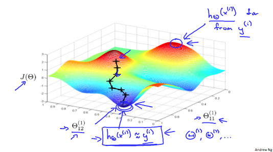
Ideally, you want $h_{\theta} (x^{(i)} \approx y^{(i)}$. This will minimize our cost function. However, keep in mind that J(Θ) is not convex and thus we can end up in a local minimum instead.